Scaling Reverse-ETL Data Pipeline

Scaling a data pipeline isn't a simple endeavor—especially when managing massive datasets and maintaining performance. In this post, we’ll take you behind the scenes to highlight the strategic improvements we've implemented to scale up our system. From handling Change Data Capture (CDC) to optimizing data processing, we’ll dive into the technical innovations that have helped us keep the system efficient, reduce costs, and ensure a smooth data flow for our users.

By Gil Omer, Prayansh Srivastava

Two years ago, we launched our Reverse-ETL solution to fill the gap of activating warehouse data natively through Segment. We initially set a limit of up to 30 million records being processed in a single sync, which was a reasonable limitation at the time.

However, over time, as the adoption of warehouse-centric CDPs grew and more companies leveraged their data warehouses for activation, the scale our customers needed grew as well.

As a result, we had to consider how to scale up our Reverse-ETL data pipeline. In our previous implementation, when the sync size exceeded 30 million records, the process would fail and display an error message, prompting the customer to adjust their setup to retrieve a smaller dataset.

This can be frustrating, as the problem may occur without warning, and fixing it can be time-consuming, potentially resulting in stale data.

Factors we considered for increased scale

  • Customer warehouse compute costs: Excessive data scans or overly complex queries can significantly increase warehouse compute costs. We were mindful of this during our decision-making process to minimize unnecessary costs for our customers while scaling.

  • Batch-based system and network error tolerance: Maintaining open connections when reading large volumes of data increases the likelihood of network failures. We developed creative approaches to handle these failures efficiently while maintaining scalability.

  • Downstream destinations restrictions and limits: We support hundreds of destinations, each with its own rate limits. Sending all the extracted data at once, would have caused overloads. We designed our system to respect these limits by batching and throttling the data transfer appropriately.

  • Data residency: We prioritize data privacy and only retain customer data for as long as necessary, unless the customer explicitly configures the pipeline to store it longer. This principle was integral to our scaling strategy, ensuring that we maintained this quality even as we grew.

Why not simply increase the limitation (or completely remove it)?

This is how our system worked before the recent changes: First, we would detect the data needed to be extracted from the warehouse. Then, we would check if there were more records to read than our limit. If so, we would fail the sync with a warning message.

So why not simply increase the limit? There are multiple reasons why continuing to raise the limit without making architectural changes is problematic, including:

Network failures:
The nature of the system is batch-based, meaning we perform operations on the data warehouse to capture data changes. We then read all the data as one batch and activate it by sending it to the connected downstream destinations.

The first issue with simply increasing the limit is the potential for network failures. For instance, if we identify 1 billion records that need to be read from the warehouse, each with hundreds of columns, reading that amount of data could take hours or even days. The likelihood of network failures during such an extended period is significant.

Service reboot:
Even if the network remains stable throughout the entire process, the service that reads the data might need to be rebooted due to deployment, auto-scaling, etc. Reading 99% of the data and then failing—only to restart the process—can result in significant delays in data delivery.

Overwhelming the data pipeline:
Scaling up by simply allowing more data to flow into the system means that the underlying services must be prepared for that increase as well. Otherwise, issues can disrupt the system. Some examples include queues getting filled up, out-of-memory failures, and noisy neighbor problems. Therefore, we had to ensure that when we scale up, we do so responsibly. 

Under the Segment hood

1. Limiting Processed Data to Maintain Stability:

The first step we took to scale up the data pipeline was to limit the maximum amount of data processed in the warehouse with each run. This step might sound counterintuitive: why add a new limit when we want to scale up? The rationale was to ensure that any amount of data we process while operating in the warehouse can be handled by our services.

This represents a change from our previous logic, where we did not implement any limitations on the amount of data processed in the warehouse. Instead, we checked if we had reached our internal limits right before starting to extract the data, and if we had, the process would fail.

Our improvements now enable us to process a larger Change Data Capture (CDC) up to 150 million records. And if we detect a CDC resultset larger than that, we limit the process to the first 150 million and queue the rest for the next scheduled sync. The key benefit here is that we can process significantly larger datasets without failure, ensuring seamless delivery of data downstream, with better reliability for our customers.
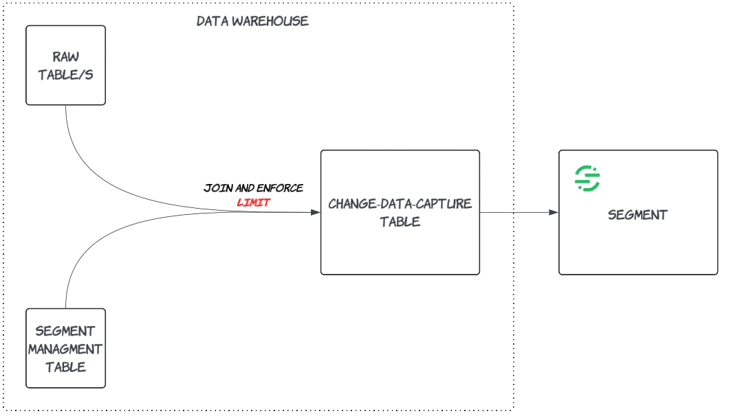
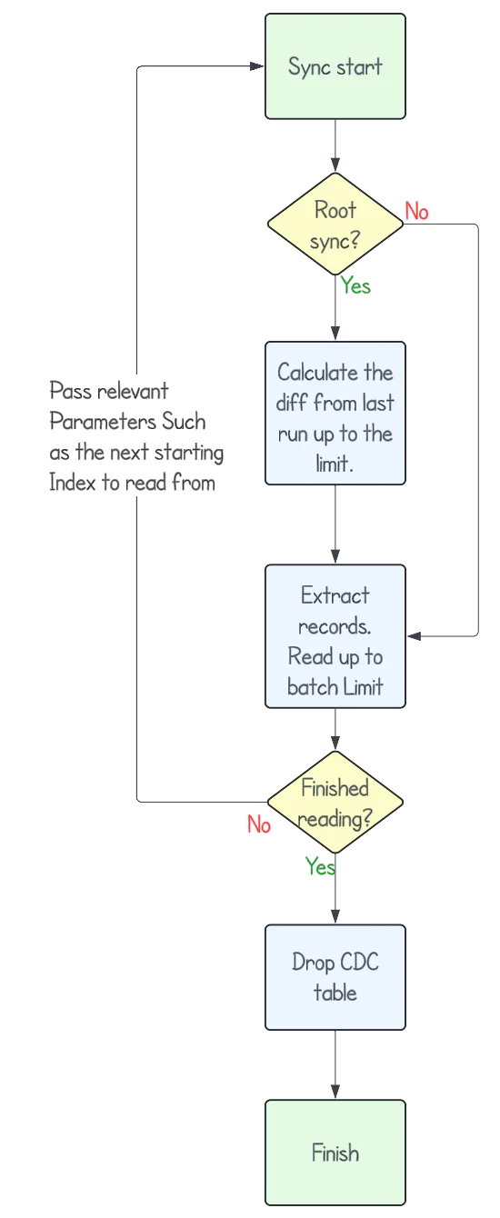
Diagram showing data warehouse flow from raw tables to change-data-capture table to segment.

Win: The system no longer fails on large data volumes, allowing continuous data processing and timely delivery.

2. Processing Data Just Once, Reducing Compute Costs:

Another significant improvement came in how we process the data. We set a high data limit per run (150 million records), but more importantly, we optimized the way data is processed and read. Initially, our system processed data in small batches, checking for CDC changes before each batch. However, after some testing, we realized we could process the entire dataset in a single pass and then read the results in batches, avoiding unnecessary computations.

The key benefit of this shift is a reduction in compute costs. Each table scan to detect CDC incurs a cost, so by minimizing the number of scans, we saved customers significant compute expenses.

Win: We reduced warehouse scans, leading to lowered costs while still handling larger data volumes efficiently.

3. Reading Data in Batches to Ensure Robustness:

After processing the CDC dataset in the warehouse, the next step is to activate the data and move it into the customer's downstream systems (e.g., Segment). One challenge we faced was the potential for failures during long-running read operations—network issues or service reboots could cause us to start over, wasting both time and compute resources.

To solve this, we started reading the data in small batches. This way, if a failure occurs, we can resume from the last successfully read batch rather than restarting the entire process. This approach also allowed us to efficiently read large datasets without needing indices (which many tables don’t have) and without incurring high compute costs from ORDER BY operations.

We used the ROW_NUMBER() function to assign row numbers to each record in the CDC dataset, allowing us to divide the data into batches.
A technical breakthrough came when we realized we could use

ROW_NUMBER() OVER (ORDER BY (SELECT NULL))

By doing that we avoid the performance penalties of ordering rows explicitly. This solution gave us the flexibility to batch reads efficiently without additional compute overhead.

Flowchart illustrating steps from starting sync, calculating differences, extracting records, to finishing sync.

Win: We implemented a robust batch-read solution that handles failures gracefully and avoids compute-intensive operations like ORDER BY, further reducing costs.

4. Automated Next Runs and Consolidated Results:

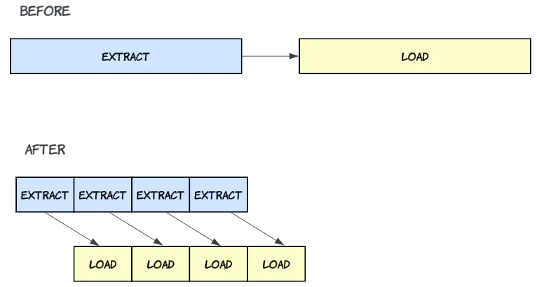
By breaking down the sync into sub-syncs, each handling the next batch, we needed a mechanism to automatically trigger the next run.

Each sub-sync knows where to pick up by referencing the last processed row index. This enables us to run multiple sub-tasks in parallel,
extracting data from the warehouse while loading it into the destination, significantly increasing throughput.

Additionally, we consolidate results from these sub-tasks to provide a cohesive view of the sync. This approach ensures that even when a large dataset is broken into smaller pieces, the final output is unified, allowing customers to track their data flow more easily.

Before and After Diagram of ETL Process Workflow

Win: We achieved parallelism between extraction and loading phases, boosting performance and ensuring seamless data processing across sub-syncs.

The Results: Smoother Data Flow, Lower Costs, and Better Scalability

With these technical improvements, we’ve managed to handle larger datasets more efficiently, reduce unnecessary compute costs, and ensure reliable data delivery. By implementing data limits, processing in batches, and utilizing parallelism, we have created a robust system that minimizes failures and reduces compute costs. These changes not only streamline the data extraction and loading phases but also ensure that our customers can rely on timely and accurate data activation. As we continue to innovate, our focus remains on delivering a seamless experience while scaling to meet growing demands.

Acknowledgements:

Huge thanks to the entire team: Gil Omer, Prayansh Srivastava, Nolan Chan, Ravi Singh, Renee Wang, Bharath Boregowda, Jon Kilroy.

The State of Personalization 2024

Our annual look at how attitudes, preferences, and experiences with personalization have evolved over the past year.

Recommended articles

Loading

Want to keep updated on Segment launches, events, and updates?